Problem

The problem presented in this assignment is to apply spatial statistics methods to get a better understanding of the spatial distribution of Emergency Medical Service (EMS) calls. These tools generally find the presence or absence of clustering/dispersion on either attribute values, the geographic location itself, or both.

Analysis Procedures

Strategies

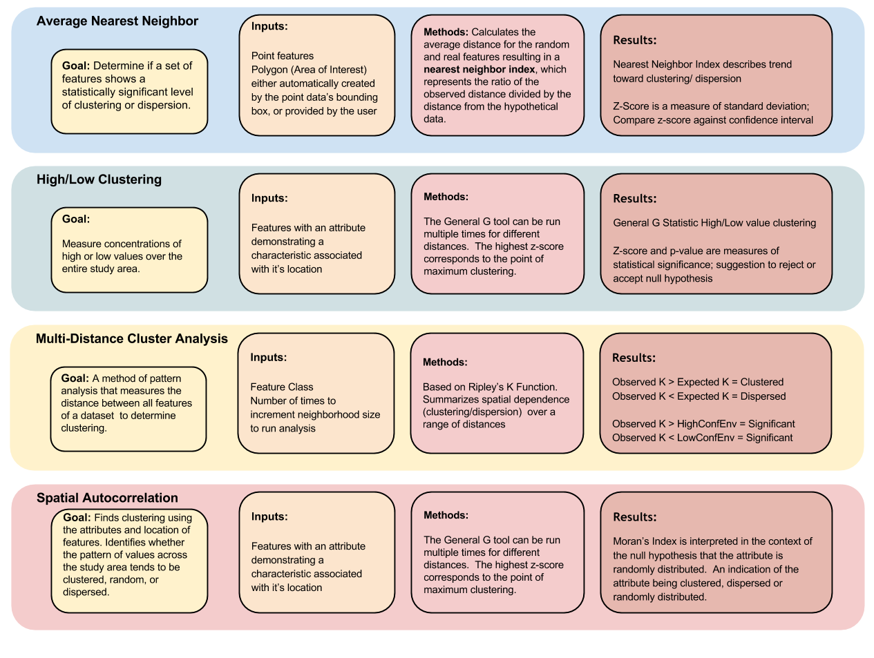
For this assignment we used the Spatial Statistics tools available in ArcGIS. We used the Average nearest neighbor tool to test for geographic clustering using an input dataset of EMS point locations, and a polygon feature representing the area of Battalion 2’s footprint. For the next exercise we used the General G statistic, which measures concentrations of high/low values over an entire study area. The third tutorial covered Ripley’s K function pattern analysis to determine clustering. The key difference between the average nearest neighbor and Ripley’s K is that the latter tests against all points in the dataset rather than just the nearest neighbor. Finally we used Moran’s I to identify clustering using attributes and geographic location.

Methods

Include a brief description in a paragraph form and a diagram that clearly communicate the procedures and overall process you used to solve the problem. Overall, this section should be a generalized description for solving the problem, which could be also used for solving other similar problems. Hence, this is NOT to be a detailed step-by-step procedure log and it should not be a click-by-click description. The diagram should also be a generalized graphical/visual representation of your workflow used to solve the problem. You may create the diagram using any software/format available, and include it as a screen capture in your text document. Ensure that the text associated with the diagram is readable. If you include separate diagrams and writeup for the four exercises, which is not necessary, it is ok if the document is longer than 2 pages.

Discussion

Difficulties Encountered

Since the tutorials associated with this assignment were step-by-step I didn’t really encounter any “blocking” problems. The one issue I had was with exercise two using the High/Low Clustering Tool. Since we were using relatively small distances each time we ran the tool using a different distance measure we got the same error: “X number of features didn’t have neighbors the statistical properties of the test are generally invalid.” The assignment suggested that we choose the result with the maximum z-score, however, this result coincided with the largest number of features that couldn’t find a neighbor within the given distance. I found these results to be the least trust-worthy.

Evaluation

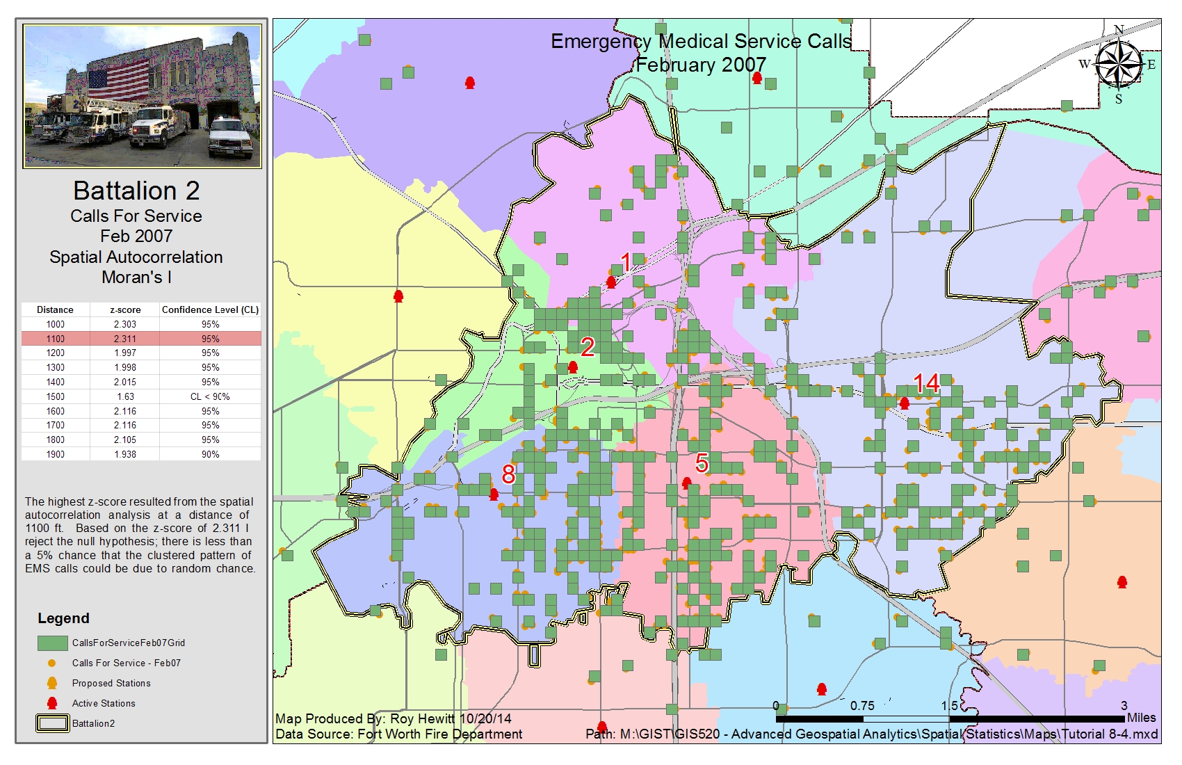
This was the first time that we were able to use statistical analysis to quantify the accuracy of our results. We were able to use the z-score and p-value of our statistical analysis to get a Confidence Level of our results. Based on these values we were able to make an educated decision whether or not to reject the null hypothesis. In statistical analysis the null hypothesis, in the case of spatial statistics, represents “Complete Spatial Randomness (CSR), either of the features themselves or of the values associated with those features.” An example of this using the Spatial Autocorrelation exercise showed that based on an input distance of 1100 feet and a z-score of 2.311 I rejected the null hypothesis. There was less than a 5% chance that the clustered pattern of EMS calls could be due to random chance.

Application & Reflection

Problem description

We need to create a density surface of Submerged Aquatic Vegetation (SAV) for several sampling locations in the Chesapeake Bay to monitor growth and recovery in response to removal of Mute Swans. Mute swans are invasive to North America and can consume up to 9 lbs of SAV a day.

Data needed

For each survey location we have randomly selected 25 survey points from a grid where we drag an SAV rake to pull up vegetation. Based on the amount of vegetation on the rake we score the location between 0 (no SAV on rake) to 4 (rake is completely covered in SAV). Additionally we need a feature class of Mute Swan occurrence locations.

Analysis procedures

For each survey location we map the GPS locations where we did SAV density measurements along with the swan occurrences. We can use these attributes with the multi-distance spatial cluster analysis to determine if mute swans and low densities of SAV are spatially related phenomena. This analysis produces a table containing expected and observed K values. A comparison of the two values suggests that the tested the SAV density and proximity of mute swans are more clustered or dispersed than a random sample. Based on the confidence interval we select we can also determine if our resluts are statistically significant by testing if the observed K value is greater than the higher confidence envelope or lower than the lower confidence envelope. If we determine that mute swans and low SAV densities are clustered we can justify a management plan that includes removing the swans from the Bay.

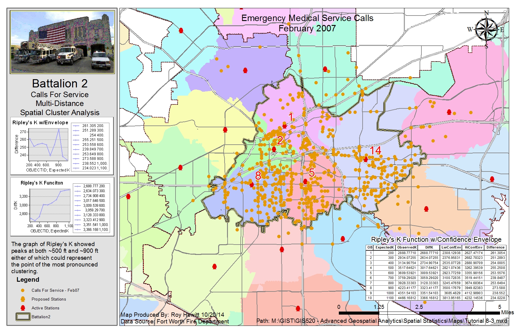
This map shows the cluster analysis for Emergency Management System (EMS) calls from Batallion 2.

This map shows the spatial autocorrelation analysis for Emergency Management System (EMS) calls from Batallion 2.