Problem

For this exercise I have been contacted by the California State Department of Natural Resources to model Bald Eagle habitat around Big Bear Lake in the San Bernardino National Forest. Rather than a traditional raster-cell based analysis I’ve been asked to conduct a fuzzy-tolerance analysis to account for the Bald Eagle’s instinctual site selection tendencies. This can often give more accurate results as animals are not bound to polygon boundaries, and do not see the world through 30 square meter raster cells.

Analysis procedures:

Strategies

I’ll once again use ArcMap’s Spatial Analysis tools for this assignment. The Spatial Analysis toolbox includes several “fuzzy” specific tools that account for uncertainty. Fuzzy overlay analyses allow us to account for uncertainty in events such as the likelihood that an animal successfully mates, or a scavenger finding a food source. Luckily the National Forest GIS staff has already prepared several layers for my analysis including distance to human disturbance, distance to water, and a reclassified landcover dataset. All input datasets are of type raster.

Methods

For each input dataset I will run the fuzzy membership tool, which reclassifies the input data to a 0 to 1. Lower numbers are less likely to be a “member of the set” or likelihood of a Bald Eagle nesting in a certain location, while higher numbers suggest a greater possibility of being a “member of the set”. Once we have a fuzzy membership layer for each of our input datasets we can overlay them to create a single fuzzy surface that accounts for human disturbance and distance to water characteristics. We use the AND operator because we want to find areas where all three criteria are met. Finally we run a second fuzzy overlay with the PRODUCT operator on the tree cover fuzzy membership layer and the result of the first fuzzy overlay analysis. This gives us our final fuzzy surface, which represents the likelihood that a Bald Eagle will nest anywhere in our study area based on our three input factors.

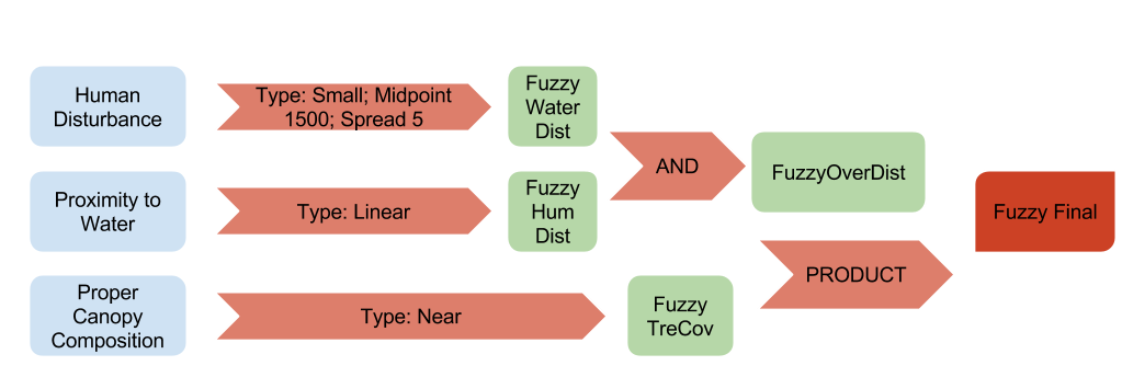
Discussion:

Difficulties Encountered

For some reason my geodatabase was corrupted after I finished my analysis. ArcMap was unable to open most of the rasters I created using the fuzzy overlay and fuzzy membership geoprocessing tools. There was no clear reason for why this happened, and I was forced to re-run the analysis to create the rasters a second time.

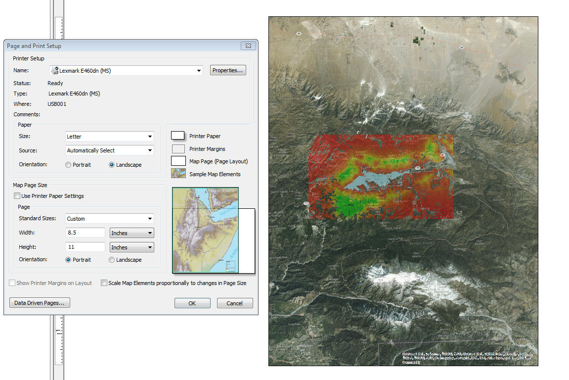
Secondly, ArcMap refused to change the orientation of my map document in layout view from Portrait to Landscape. I went into the print/page view settings and changed the orientation, but it was never updated in the layout view. I tried saving, closing ArcMap then re-opening the map document but nothing I tried worked. The shape of Big Bear Lake lends itself to a landscape view to make better use of all available space.

Evaluation

Describe the procedure you used to check appropriates of the procedures and/or accuracy of the results. These procedures are not provided with the assignment description, which will be very varied based on the nature of the problem solved, but you should develop a practice of double checking the results of your work and methods selected to perform analysis. For example, you could perform visual check, perform visual comparison of few layers, review the attribute table output, or use another method to perform the same analysis to judge the accuracy of the results and/or appropriateness of methods used. Some exercises will be straightforward and will require fewer checks, while others may require more a extensive approach.

I did a visual analysis of areas that had higher scores for the initial fuzzy membership rasters. Both times I ran the fuzzy overlay geoprocessing tool I used additive (SUM, PRODUCT) overlay types I operated under the supposition that green areas in the input datasets that overlapped would result in green areas (high probability) for the overlay analysis.

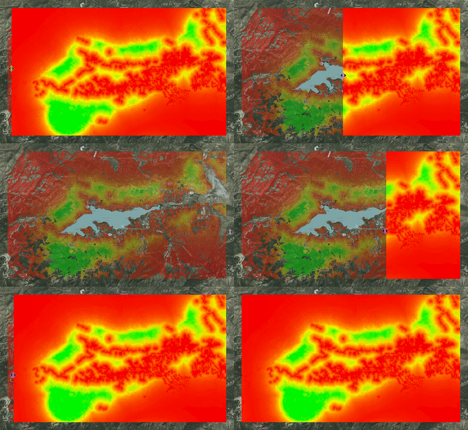
In this animated image you can see me swipe away the intermediate fuzzy overlay to show the final model. I used a second fuzzy overlay with the intermediate overlay and the tree fuzzy membership raster. Areas in green from both inputs are represented as green in my final output.

Application and Reflection

Fuzzy overlay analysis is probably the best analysis to apply in natural resource applications. The whole purpose of GIS layers is to accurately represent some sort of geographic phenomena. In the world of natural resources that could be landcover, paths/roads, temperature, precipitation, etc. The problem is that we have only two ways to represent these environmental factors: vector and raster datasets. Unfortunately, in the real-world, plants and animals live their lives far removed from such cut and dry points, lines, polygons, and raster cells. As such a fuzzy overlay approach to modeling the natural environment can often provide more accurate models.

For my work with the U.S. Fish & Wildlife Service on the Chesapeake Bay Nutria Eradication Program we sought to eliminate nutria, a marsh rodent, from the entire estuary. I joined the team late in the game as a GIS analyst after the team of trappers had already eliminated the majority of the Chesapeake Bay population. The remaining population generally existed in areas that had not recently been surveyed, and marginal habitats. As such it was difficult to model where we could find the remaining nutria based on environmental factors alone. Luckily the team rigorously recorded their daily survey tracks showing which portions of the Bay had been surveyed over certain time spans.

Problem description

Create a model that quantifies the probability of encountering a nutria during a field survey.

Data needed

The data needed in this analysis include a feature class of all past surveys including the type of survey conducted. Each type of survey has a different probability of encountering a nutria so they must be weighted differently. Second we need a raster landcover dataset that allows us to identify particular habitats where nutria are known to occur more often than in marginal habitats.

Analysis procedures

With the use of fuzzy overlay modeling I can take into account the location, type of survey (foot, detector dog, shoreline boat), and how recent the survey was conducted along with more traditional environmental factors like vegetation type, density, and salinity. More recent surveys that resulted in a detection would suggest other surveys in that area would also result in detection. Likewise if a recent survey did not return any detections it would suggest that another survey in that area would be unlikely to result in a detection.

For each layer I need to use the fuzzy membership geoprocessing tool to create a probability surface. I would then use the fuzzy overlay tool to combine the vegetation raster with the raster of past surveys and salinity surface using the AND overlay type because the combined evidence of each of the factors should have a high value to suggest a high probability of detecting another nutria.

It’s important to realize that this type of analysis wouldn’t tell us the most suitable habitat for the nutria, but instead would suggest the most likely areas our field staff would encounter a nutria. This is incredibly useful information when the population is reduced to the point that staff may go weeks without encountering a nutria.

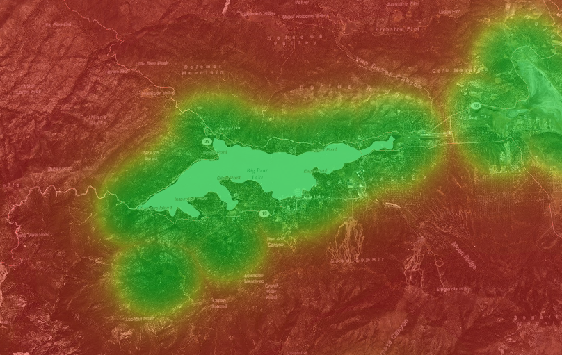
This image shows the fuzzy membership raster for the proximity to water input raster.

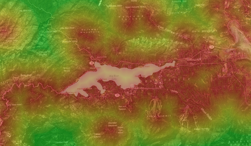
This image shows the fuzzy membership raster for the proximity to human disturbance input raster.

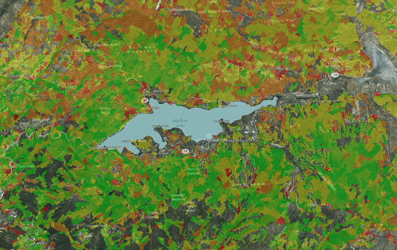
This image shows the fuzzy membership raster for the proximity to landcover input raster.

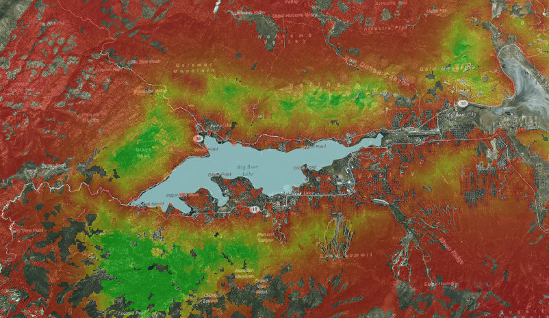
This image shows the final fuzzy overlay model output. It was created by running a fuzzy overlay on the intermediate FuzzyOverDist raster and the FuzzyTreeCov fuzzy membership raster.